|
|
New facebook book page with info on my updates and new developments in science/engineering. |
Kalman Filter: "Cause knowing is half the battle" - GI Joe
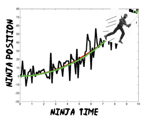
As mentioned in the bayesian discussion, when predicting future events we not only include our current experiences, but also our past knowledge. Sometimes, that past knowledge is so good that we have a very clear model of how thinks should pan out. For example, when you run and reach out to catch a ball, it's only because you have a very good model of how ballistic objects move on earth that you can catch it (or at least not get hit by it). The Kalman filter is an optimized quantitative expression of this kind of system. By optimally combining a expectation model of the world with prior and current information, the kalman filter provides a powerful way to use everything you know to build an accurate estimate of how things will change over time (figure shows noisy observation (black) and good tracking (green) of accelerating Ninja aka Snake-eyes).
|
These tutorials are fueled by coffee and Ramen. If you would like to see more sooner, plz make a small donation. thx! :)
|

|
| studentdave_kalmanfilter_code.m |
Bayesian Ninja Consulting!
Do you need help implementing an idea? Do you need code? Do you need help understanding some concepts? Shoot me an email at [email protected] or submit to my feedback bar on the homepage! happy quail hunting!
% written by StudentDave
%for licensing and usage questions
%email scienceguy5000 at gmail. com
%Bayesian Ninja tracking Quail using kalman filter
clear all
%% define our meta-variables (i.e. how long and often we will sample)
duration = 10 %how long the Quail flies
dt = .1; %The Ninja continuously looks for the birdy,
%but we'll assume he's just repeatedly sampling over time at a fixed interval
%% Define update equations (Coefficent matrices): A physics based model for where we expect the Quail to be [state transition (state + velocity)] + [input control (acceleration)]
A = [1 dt; 0 1] ; % state transition matrix: expected flight of the Quail (state prediction)
B = [dt^2/2; dt]; %input control matrix: expected effect of the input accceleration on the state.
C = [1 0]; % measurement matrix: the expected measurement given the predicted state (likelihood)
%since we are only measuring position (too hard for the ninja to calculate speed), we set the velocity variable to
%zero.
%% define main variables
u = 1.5; % define acceleration magnitude
Q= [0; 0]; %initized state--it has two components: [position; velocity] of the Quail
Q_estimate = Q; %x_estimate of initial location estimation of where the Quail is (what we are updating)
QuailAccel_noise_mag = 0.05; %process noise: the variability in how fast the Quail is speeding up (stdv of acceleration: meters/sec^2)
NinjaVision_noise_mag = 10; %measurement noise: How mask-blinded is the Ninja (stdv of location, in meters)
Ez = NinjaVision_noise_mag^2;% Ez convert the measurement noise (stdv) into covariance matrix
Ex = QuailAccel_noise_mag^2 * [dt^4/4 dt^3/2; dt^3/2 dt^2]; % Ex convert the process noise (stdv) into covariance matrix
P = Ex; % estimate of initial Quail position variance (covariance matrix)
%% initize result variables
% Initialize for speed
Q_loc = []; % ACTUAL Quail flight path
vel = []; % ACTUAL Quail velocity
Q_loc_meas = []; % Quail path that the Ninja sees
%% simulate what the Ninja sees over time
figure(2);clf
figure(1);clf
for t = 0 : dt: duration
% Generate the Quail flight
QuailAccel_noise = QuailAccel_noise_mag * [(dt^2/2)*randn; dt*randn];
Q= A * Q+ B * u + QuailAccel_noise;
% Generate what the Ninja sees
NinjaVision_noise = NinjaVision_noise_mag * randn;
y = C * Q+ NinjaVision_noise;
Q_loc = [Q_loc; Q(1)];
Q_loc_meas = [Q_loc_meas; y];
vel = [vel; Q(2)];
%iteratively plot what the ninja sees
plot(0:dt:t, Q_loc, '-r.')
plot(0:dt:t, Q_loc_meas, '-k.')
axis([0 10 -30 80])
hold on
pause
end
%plot theoretical path of ninja that doesn't use kalman
plot(0:dt:t, smooth(Q_loc_meas), '-g.')
%plot velocity, just to show that it's constantly increasing, due to
%constant acceleration
%figure(2);
%plot(0:dt:t, vel, '-b.')
%% Do kalman filtering
%initize estimation variables
Q_loc_estimate = []; % Quail position estimate
vel_estimate = []; % Quail velocity estimate
Q= [0; 0]; % re-initized state
P_estimate = P;
P_mag_estimate = [];
predic_state = [];
predic_var = [];
for t = 1:length(Q_loc)
% Predict next state of the quail with the last state and predicted motion.
Q_estimate = A * Q_estimate + B * u;
predic_state = [predic_state; Q_estimate(1)] ;
%predict next covariance
P = A * P * A' + Ex;
predic_var = [predic_var; P] ;
% predicted Ninja measurement covariance
% Kalman Gain
K = P*C'*inv(C*P*C'+Ez);
% Update the state estimate.
Q_estimate = Q_estimate + K * (Q_loc_meas(t) - C * Q_estimate);
% update covariance estimation.
P = (eye(2)-K*C)*P;
%Store for plotting
Q_loc_estimate = [Q_loc_estimate; Q_estimate(1)];
vel_estimate = [vel_estimate; Q_estimate(2)];
P_mag_estimate = [P_mag_estimate; P(1)]
end
% Plot the results
figure(2);
tt = 0 : dt : duration;
plot(tt,Q_loc,'-r.',tt,Q_loc_meas,'-k.', tt,Q_loc_estimate,'-g.');
axis([0 10 -30 80])
%plot the evolution of the distributions
figure(3);clf
for T = 1:length(Q_loc_estimate)
clf
x = Q_loc_estimate(T)-5:.01:Q_loc_estimate(T)+5; % range on x axis
%predicted next position of the quail
hold on
mu = predic_state(T); % mean
sigma = predic_var(T); % standard deviation
y = normpdf(x,mu,sigma); % pdf
y = y/(max(y));
hl = line(x,y,'Color','m'); % or use hold on and normal plot
%data measured by the ninja
mu = Q_loc_meas(T); % mean
sigma = NinjaVision_noise_mag; % standard deviation
y = normpdf(x,mu,sigma); % pdf
y = y/(max(y));
hl = line(x,y,'Color','k'); % or use hold on and normal plot
%combined position estimate
mu = Q_loc_estimate(T); % mean
sigma = P_mag_estimate(T); % standard deviation
y = normpdf(x,mu,sigma); % pdf
y = y/(max(y));
hl = line(x,y, 'Color','g'); % or use hold on and normal plot
axis([Q_loc_estimate(T)-5 Q_loc_estimate(T)+5 0 1]);
%actual position of the quail
plot(Q_loc(T));
ylim=get(gca,'ylim');
line([Q_loc(T);Q_loc(T)],ylim.','linewidth',2,'color','b');
legend('state predicted','measurement','state estimate','actual Quail position')
pause
end
